Please Note: This article is written for users of the following Microsoft Excel versions: 2007, 2010, 2013, and 2016. If you are using an earlier version (Excel 2003 or earlier), this tip may not work for you. For a version of this tip written specifically for earlier versions of Excel, click here: Creating 3-D Formatting for a Cell.
Written by Allen Wyatt (last updated September 24, 2020)
This tip applies to Excel 2007, 2010, 2013, and 2016
Do you want the formatting of a cell to "stand out" from the surrounding cells? It's rather easy to do, once you understand how to create the illusion of three dimensions. Follow these steps:
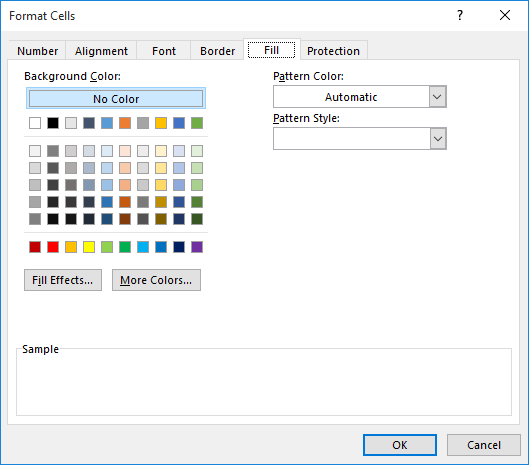
Figure 1. The Fill tab of the Format Cells dialog box.

Figure 2. The Border tab of the Format Cells dialog box.
The cell you selected in step 1 should now look as if it is "raised" off the worksheet around it. You can accentuate the effect even more if you apply a background color to the cells that surround the one that you want to look raised.
ExcelTips is your source for cost-effective Microsoft Excel training. This tip (12143) applies to Microsoft Excel 2007, 2010, 2013, and 2016. You can find a version of this tip for the older menu interface of Excel here: Creating 3-D Formatting for a Cell.
Solve Real Business Problems Master business modeling and analysis techniques with Excel and transform data into bottom-line results. This hands-on, scenario-focused guide shows you how to use the latest Excel tools to integrate data from multiple tables. Check out Microsoft Excel 2013 Data Analysis and Business Modeling today!
Need a line through the middle of your text? Use strikethrough formatting, which is easy to apply using the Format Cells ...
Discover MoreYou can spend a lot of time getting the formatting in your worksheets just right. If you want to protect an element of ...
Discover MoreIf you need to change fonts used in a lot of different workbooks, the task can be daunting, if you need to do it ...
Discover MoreFREE SERVICE: Get tips like this every week in ExcelTips, a free productivity newsletter. Enter your address and click "Subscribe."
2020-09-24 18:18:36
Ronmio
I would suggest using a medium gray for the bottom and right borders. That will look more like a shadow effect than black will. Here are illustration using all three border widths.
(see Figure 1 below)
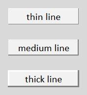
Figure 1. 3-D Examples
2020-09-24 10:58:51
Donald
I tried this Tip in my Office 365 Excel and wasn't impressed with it at all. I tried 5 cells of varying sizes and none of them had that '3D' look to it. But, on the other habd, this has increased my knowledge of Excel. So, thanks, Allen, for the tip. I look forward to others that you may post.
2017-02-06 13:28:51
Brian
The tip works nicely. Spend a coupla minutes and make a little table using the tip. As a variation of this tip, rather than use white and black for the edges, use lighter and darker shades of the cell fill color to get the raised effect. You can reverse the colors to get a sunken effect.
2017-02-06 08:30:57
Russell
Not what I expected based on the Excel Tips Newsletter description, but does result in a nice 3D button effect.
2017-02-06 08:07:22
Bill Korebein
Not a useful tip without a picture of the result
2017-02-06 05:33:13
Ken Varley
Disappointed with this tip.
You showed a picture of raised triangles in your letter, not a button
2017-02-04 13:25:53
Carlos
not very clear - need picture of the result
Got a version of Excel that uses the ribbon interface (Excel 2007 or later)? This site is for you! If you use an earlier version of Excel, visit our ExcelTips site focusing on the menu interface.
FREE SERVICE: Get tips like this every week in ExcelTips, a free productivity newsletter. Enter your address and click "Subscribe."
Copyright © 2024 Sharon Parq Associates, Inc.
 Please Note:
This article is written for users of the following Microsoft Excel versions: 2007, 2010, 2013, and 2016. If you are using an earlier version (Excel 2003 or earlier), this tip may not work for you. For a version of this tip written specifically for earlier versions of Excel, click here:
Please Note:
This article is written for users of the following Microsoft Excel versions: 2007, 2010, 2013, and 2016. If you are using an earlier version (Excel 2003 or earlier), this tip may not work for you. For a version of this tip written specifically for earlier versions of Excel, click here:
Comments